Spectral Analysis Methodology · The Exoplanet Codex

Section 01

Data Acquisition

All spectra are retrieved from the ESO Science Archive, which provides public access to reduced data products after a 12-month proprietary period.

Primary Instrument: HARPS

Parameter	Value	Notes
Telescope	ESO 3.6m, La Silla	Chile
Spectral Resolution	R ~ 115,000	vs. R ~ 42,000 in Schmitt (2010)
Wavelength Coverage	3780 – 6910 Å	Two arms: blue + red
Mode	HAM	High Accuracy Mode
Data Product	S1D	1D merged, wavelength-calibrated, barycentric-corrected
Archive Epochs (55 Cnc A)	88 spectra	All used after quality inspection

Instrument Suite

Instrument	Facility	Wavelength Range	Resolution	Usage
HARPS	ESO 3.6m, La Silla, Chile	3780 – 6910 Å (optical)	R ~ 115,000	Primary instrument for all FGK/M dwarf targets — optical stellar spectra
HST/STIS	Hubble Space Telescope — Space Telescope Imaging Spectrograph	~1150 – 10,000 Å (UV + optical)	Varies by grating	UV oxygen lines inaccessible from ground. Gratings used: G140M, G750L, G430L (55 Cnc A); E140H, E140M, E230H, E230M (Alpha Cen A)
HST/COS	Hubble Space Telescope — Cosmic Origins Spectrograph	~1150 – 3200 Å (far-UV)	High sensitivity far-UV	Far-UV spectra where available; high sensitivity for faint far-UV features

Multi-Wavelength Strategy

Optical HARPS spectra cover the majority of target elements. HST UV coverage (STIS + COS) unlocks element lines that are blocked by Earth's atmosphere — critical for N, O, C UV transitions and for cross-validating ground-based oxygen measurements. HST data retrieved from MAST (Mikulski Archive for Space Telescopes, mast.stsci.edu).

Target Selection Criteria

1Confirmed exoplanet host (NASA Exoplanet Archive)
2FGK spectral type (T_eff 4000–7000 K) — ATLAS9 grid; M dwarfs (T_eff < 4000 K) use MARCS spherical grid
3Main sequence dwarf (log g > 3.8) — plane-parallel atmosphere valid
4V < 9 mag — sufficient HARPS S/N achievable
5Multiple HARPS epochs available for co-adding
6Not a spectroscopic binary

Spectrum Co-Adding (55 Cnc A — 88 Epochs)

S/N_coadd ≈ √88 × 100 ≈ 940 per pixel at 6000 Å

This makes phosphorus (P I 6034 Å, EW ~ 12 mÅ) and lithium (Li I 6707 Å, EW ~ 3 mÅ) accessible — both invisible in a single exposure.

Element	Line EW	Single epoch S/N 100	Co-add S/N 940
Fe I	~80 mÅ	Yes (40σ)	Yes (400σ)
Ca I	~40 mÅ	Yes (20σ)	Yes (200σ)
P I	~12 mÅ	No (6σ — marginal)	Yes (60σ)
Li I	~3 mÅ	No (1.5σ)	Yes (15σ)

Radial Velocity Correction

Each spectrum is shifted to the stellar rest frame before co-adding: λ_rest = λ_obs / (1 + v_r / c). 55 Cnc A hosts 5 planets with total RV variation up to ±100 m/s — equivalent to ~0.002 Å at 6000 Å. Uncorrected co-adding blurs line profiles at the 0.2-pixel level.

Section 02

Stellar Model Atmosphere

We use the ATLAS9 one-dimensional, plane-parallel, LTE model atmosphere grid of Castelli & Kurucz (2003) — the current standard for FGK main-sequence dwarfs.

ATLAS9 Model Assumptions

Assumption	Plain English	Valid For
1D plane-parallel geometry	Atmosphere modeled as flat parallel layers	Main-sequence dwarfs (log g > 3.5)
LTE	Each layer in thermal equilibrium — Boltzmann/Saha distributions	Dense collision-dominated FGK photospheres
Opacity Distribution Functions	Millions of line opacities treated statistically for efficiency	All spectral types

Cross-validation: key results also run through MARCS grid (Gustafsson et al. 2008). ATLAS9 vs. MARCS differences are typically < 0.03 dex for FGK dwarfs and are included in the systematic uncertainty budget.

55 Cancri A Model Parameters

Parameter	Symbol	Value	Uncertainty	Source
Effective temperature	T_eff	5196 K	± 24 K	CHARA interferometry — von Braun et al. 2011, ApJ 740, 49
Surface gravity	log g	4.41	± 0.02	CHARA interferometry — von Braun et al. 2011
Metallicity	[Fe/H]	+0.32	± 0.02	Spectroscopic self-consistency (§4)
Microturbulence	ξ	~0.9 km/s	± 0.1 km/s	Fe I EW self-consistency (§4)

Section 03

Atomic Data: Line List

All atomic line data are loaded from external, version-controlled CSV files. No wavelengths or log gf values are hardcoded in pipeline software — ensuring full traceability.

VALD3 Query Settings

Setting	Value	Notes
Query type	Extract Stellar	Filters by predicted line depth for given stellar parameters
Wavelength range	3780 – 6910 Å	Matches HARPS coverage
Depth threshold	≥ 1% of continuum	Removes lines too weak to measure
Access method	FTP (required)	HTTP truncates large requests — use vald.astro.uu.se FTP
Format	Long format	Includes broadening parameters (γ_vdW)

⚠ FTP Required for Full Line List

The VALD3 web interface truncates output for large requests. Queries covering the full HARPS range with 27 target elements require FTP access to retrieve the complete line list. Register at vald.astro.uu.se for a free academic FTP account.

NIST Quality Grades

Grade	log gf Uncertainty	Usage Policy
A+	< 1%	Full science use
A	< 3%	Full science use
B	< 10%	Science use, flagged in uncertainty budget
C	< 25%	Excluded from primary results
D	> 25%	Excluded entirely

Target Element List — 27 Elements

Priority	Element	Symbol	Group	Scientific Significance
1	Iron I	Fe I	Iron peak	[Fe/H] calibration, T_eff constraint
1	Iron II	Fe II	Iron peak	log g constraint via ionization equilibrium
1	Carbon	C	CHNOPS	C/O ratio — carbon vs. oxygen-rich planet mineralogy
1	Oxygen	O	CHNOPS	C/O ratio; most abundant metal in rocky planets
1	Magnesium	Mg	Alpha	Mg/Si ratio — mantle mineralogy (olivine vs. pyroxene)
1	Silicon	Si	Alpha	Primary rocky planet building block
1	Calcium	Ca	Alpha	Alpha element tracer; strong optical lines
1	Titanium	Ti	Alpha	Galactic chemical evolution tracer; perovskite in mantles
1	Nickel	Ni	Iron peak	Rocky planet core composition; Fe/Ni ratio
1	Sodium	Na	Bio-significant	Biological tracer; Na D doublet
1	Phosphorus	P	CHNOPS	Limiting nutrient for life; varies 10× across FGK stars
1	Sulfur	S	CHNOPS/Alpha	Life-essential volatile; disk chemistry tracer
2	Nitrogen	N	CHNOPS	Life-essential; difficult optical lines
2	Cobalt	Co	Iron peak	Fe peak nucleosynthesis tracer
2	Chromium	Cr	Iron peak	Type Ia vs. Type II SNe tracer via Cr/Fe
2	Aluminum	Al	Rocky planet	Refractory element; crustal composition
2	Potassium	K	Bio-significant	Life-essential; difficult lines
2	Barium	Ba	s-process	AGB star enrichment history
2	Yttrium	Y	s-process	Stellar age chemical clock (Y/Mg ratio)
2	Vanadium	V	Iron peak	Enzyme cofactor; nucleosynthesis tracer
2	Copper	Cu	Iron peak	Odd-Z iron-peak tracer; bio-essential; Cu I 5105/5218 Å
3	Manganese	Mn	Iron peak	Odd-Z nucleosynthesis; metallicity-dependent
3	Scandium	Sc	Light iron peak	Odd-even nucleosynthesis effect
3	Lithium	Li	Age indicator	Stellar age constraint; depletes with time
3	Europium	Eu	r-process	Neutron star merger enrichment history
3	Zirconium	Zr	s-process	Refractory s-process tracer
3	Strontium	Sr	s-process	Light s-process anchor; completes Sr/Y/Ba/Zr picture

Special Line Handling

Line	Issue	Treatment
[O I] 6300.304 Å	Blended with Fe I + Ni I 6300.336 Å	Ni blend subtracted using measured Ni abundance; no NLTE correction (forbidden line)
O I 7771–7775 Å triplet	Large NLTE corrections (−0.2 to −0.4 dex)	Amarsi et al. (2021) grid; cross-checked against [O I] 6300 Å
Na I D 5890/5896 Å	Strong — damping wings + NLTE	Voigt profile fit; Lind et al. (2011) correction (~−0.07 dex)
P I 6034/6043 Å	Very weak — requires S/N > 300	Only accessible in co-added spectrum; upper limit if < 3σ
C I 5380 Å	High χ (7.7 eV) — T_eff sensitive	Cross-validated against C I 5052 Å; Amarsi et al. (2019) NLTE correction

Section 04

Spectral Analysis

Before measuring elemental abundances, the spectrum is continuum-normalized and stellar parameters (T_eff, log g, ξ) are verified through self-consistency checks on Fe I and Fe II lines.

Continuum Normalization

1Identify continuum anchor windows — regions free of significant absorption for the target's stellar parameters (Barklem & Aspelund-Johansson 2005).
2For metal-rich stars ([Fe/H] > +0.2), use the ATLAS9 model continuum as additional reference in crowded regions (5000–5400 Å).
3Fit a Chebyshev polynomial (degree 3) through anchor points with iterative 3σ sigma-clipping.
4Divide observed spectrum by the fitted continuum.
5Verify: σ < 0.005 (0.5% of continuum) in clean windows before proceeding.

Challenge for 55 Cancri A

At [Fe/H] = +0.32, the spectrum is significantly more crowded than solar. The 5000–5400 Å region has very high Fe I line density. The ATLAS9 model continuum is weighted more heavily here to avoid over-fitting through shallow absorption features.

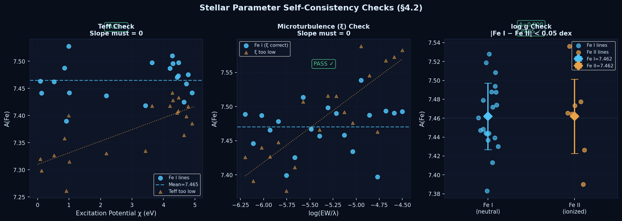
Stellar Parameter Self-Consistency

Parameter	Diagnostic	Convergence Criterion
T_eff	Fe I abundance vs. excitation potential χ	\|∂[Fe/H]/∂χ\| < 0.01 dex/eV — requires ≥ 20 Fe I lines spanning χ = 0.5–5.0 eV
ξ (microturbulence)	Fe I abundance vs. reduced EW log(EW/λ)	\|∂[Fe/H]/∂log(EW/λ)\| < 0.01 dex per unit
log g	Ionization equilibrium: A(Fe I) vs. A(Fe II)	\|A(Fe I) − A(Fe II)\| < 0.05 dex

All three constraints must be simultaneously satisfied. Convergence typically takes 3–5 iterations starting from interferometric values.

Three self-consistency diagnostic plots for 55 Cancri A — **Figure 5.** Self-consistency diagnostics for 55 Cancri A. Left: Fe I abundance vs. χ — zero slope confirms T_eff. Centre: Fe I vs. log(EW/λ) — zero slope confirms ξ. Right: Fe I vs. Fe II agreement confirms log g.

EW Measurement Quality Thresholds

Criterion	Requirement	Action if Failed
EW minimum	> 5 mÅ	Below detection — report upper limit
EW maximum	< 300 mÅ	Saturated — exclude from LTE analysis
Fit quality (χ²_red)	< 2.0	Refit or exclude
Line S/N	> 5	Exclude
Center shift	< 0.05 Å from VALD/NIST	Flag — possible misidentification

Section 05

Line Profiles

The correct line profile model depends on line strength. Gaussian fits work well for weak lines; strong lines with pressure-broadened wings require Voigt profiles.

Gaussian vs. Lorentzian vs. Voigt

Profile	Appropriate For	Physics	EW Rule
Gaussian	Weak lines EW < 80 mÅ	Thermal + instrumental broadening	≈ Voigt (< 1% difference) in this regime
Lorentzian	Theoretical damping wings only	Pressure broadening (van der Waals)	Overestimates core depth — not used alone
Voigt	All line strengths	Gaussian core convolved with Lorentzian wings	Required for EW > 150 mÅ

Always fitted with Voigt profiles: Na D doublet, Mg b triplet (5167–5184 Å), Ba II 5853 Å, Ca H&K (3934/3968 Å).

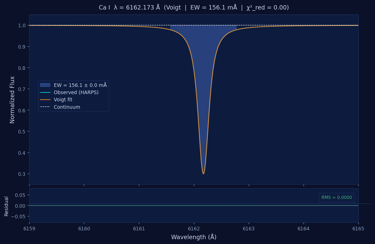
Figure 1. Ca I 6162.17 Å profile — Gaussian (dashed) vs. Voigt (solid) fit. The Gaussian underestimates pressure-broadened wings, leading to ~15% EW error for this line.

Worked Example: Na I D1 (5895.92 Å)

The Na I D doublet was first observed in the Sun by Fraunhofer (1814) and identified as sodium by Kirchhoff & Bunsen (1859). For 55 Cnc A ([Fe/H] = +0.32), the lines are especially deep due to enhanced sodium abundance.

1Locate: Extract ±5 Å around 5895.92 Å after RV correction. D1 and D2 are separated by ~6 Å, well-resolved at R~115,000.
2Choose profile: Na D EW ~ 450–550 mÅ → damping regime → Voigt required. Gaussian would underestimate EW by ~25%, causing ~0.2 dex error in [Na/H] — larger than the entire uncertainty budget.
3Measure EW: Numerical integration over fitted Voigt profile. EW = ∫(1 − F(λ)/F_c) dλ, expressed in mÅ.
4Uncertainty: Primary limit is continuum placement, not photon noise. σ_EW ≈ σ_cont × window × 1000 ≈ 0.005 × 6.0 × 1000 ≈ 30 mÅ (~6% relative).
5Atomic data: λ = 5895.924 Å (NIST A+), χ = 0.000 eV (ground state), log gf = −0.184 (NIST A), γ_vdW = −7.530 (Barklem 2000). Input to iSpec/Turbospectrum.
6NLTE correction: −0.07 ± 0.02 dex (Lind et al. 2011) for these parameters. Expected result: [Na/H] ≈ +0.34 to +0.44, [Na/Fe] ≈ +0.02 to +0.12 (near-solar ratio).

Figure 2. Na I D1 5895.92 Å in 55 Cnc A co-added spectrum. Solid: Voigt fit (EW ~ 500 mÅ). Dashed: Gaussian fit for comparison — note the wing underestimate. Bottom: residuals.

Section 06

Abundance Derivation

From equivalent width to photospheric abundance — via the curve of growth, iSpec/Turbospectrum radiative transfer, and solar normalization to Asplund et al. (2021).

The Curve of Growth

Regime	EW Range	Behavior	Notes
Linear	< ~50 mÅ	EW ∝ N (number of absorbing atoms)	Direct proportionality — preferred
Flat (saturation)	~50–150 mÅ	EW grows slowly with abundance	Sensitive to microturbulence ξ
Damping	> ~150 mÅ	EW ∝ √N (pressure-broadened wings)	Requires accurate γ_vdW; Voigt fit only

Solar Normalization

[X/H] = A(X)_star − A(X)_sun · [X/Fe] = [X/H] − [Fe/H]

Schmitt (2010) — Predecessor Study

Solar reference: Lodders (2003)

A(Fe)☉ = 7.50

Instrument: ELODIE (R ~ 42,000)

The Exoplanet Codex (2026)

Solar reference: Asplund et al. (2021)

A(Fe)☉ = 7.46 (−0.04 dex revision)

Instrument: HARPS (R ~ 115,000)

Key Science Ratios

Ratio	Threshold	Interpretation	Solar Value
C/O	0.8	Below: silicate/oxide minerals (Earth-like). Above: SiC, graphite — possible diamond interior	0.55
Mg/Si	1.0	Above: olivine-dominated mantle (Mg₂SiO₄). Below: pyroxene-dominated (MgSiO₃)	1.05
Fe/Si	—	Iron core mass fraction predictor for rocky planets	0.86 (mass)
[α/Fe]	—	High at low [Fe/H] = old star formed before Type Ia SNe Fe enrichment	~0.0
CHNOPS Index	vs. Redfield ratio	C:N:O:P:S ratios vs. marine organism composition — habitability indicator	1.0 (reference)

Section 07

Uncertainty Analysis

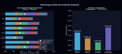
The uncertainty budget follows the Type A / Type B framework of the JCGM Guide to the Expression of Uncertainty in Measurement (GUM) — consistent with precision metrology practice.

Type A — Statistical (Random)

Source	Estimation Method	Typical Magnitude
Photon noise on EW	Covariance matrix of Gaussian/Voigt fit	σ_EW ≈ 1.5 × FWHM / S/N
Line-to-line scatter	σ / √N for N lines of same element	~0.02 – 0.05 dex
Continuum placement	Repeat normalization, vary anchor points	~0.01 – 0.03 dex

Type B — Systematic (Non-Random)

Source	Estimation Method	Typical Magnitude
ΔT_eff = ±50 K	Re-run abundances at T_eff ± 50 K	±0.05 – 0.10 dex
Δlog g = ±0.1	Re-run at log g ± 0.1	±0.02 – 0.05 dex
Δξ = ±0.1 km/s	Re-run at ξ ± 0.1	±0.03 – 0.06 dex
log gf uncertainty	NIST grade (A: 3%, B: 10%)	~0.02 – 0.05 dex
NLTE corrections	Uncertainty on correction grids	~0.02 – 0.08 dex
1D vs. 3D models	Compare ATLAS9 vs. MARCS	~0.03 – 0.10 dex (C, O)
Continuum (systematic)	Model-based vs. polynomial normalization	~0.02 – 0.05 dex

σ_total = √(σ_A² + σ_Teff² + σ_logg² + σ_ξ² + σ_loggf² + σ_NLTE²)

O I / Ni I Blend at 6300 Å

The dominant source of published C/O ratio discrepancies for 55 Cnc A (Teske et al. 2013). The Ni I 6300.336 Å contribution is calculated from our measured Ni abundance and subtracted. Its uncertainty propagates into σ(C/O) as a correlated term.

Tornado chart showing uncertainty contribution per source for priority-1 elements — **Figure 4.** Uncertainty budget tornado chart for 55 Cnc A. Each bar shows the contribution of one source to σ_total. T_eff dominates for most elements; NLTE corrections dominate for C and O.

Section 08

Data Model

The pipeline processes each star from raw ESO archive FITS files to final abundance tables through six sequential stages, each with well-defined input and output schemas.

Multi-Target Dataset Summary

Target	HARPS S1D	HST Observations	HST Gratings	Program / PI
Solar (calibrator)	10 spectra	—	—	ESO 1102.D-0954(A) · PI: Dumusque (U. Geneva) · Direct solar feed, SNR 306–309
55 Cancri A	88 spectra	STIS	G140M, G750L, G430L, E230M	Multiple programs · MAST archive
Alpha Centauri A	75 spectra	111 observations	E140H, E140M, E230H, E230M	Multiple programs · MAST archive

Solar Dataset Note

The solar spectra are direct solar feed observations — the Sun itself, not asteroid-reflected sunlight. ESO Program 1102.D-0954(A), PI Xavier Dumusque (University of Geneva). The high SNR (306–309 per exposure) allows validation of weak lines including P I 6034 Å and Li I 6707 Å before touching science targets.

Pipeline Data Flow

Pipeline flow diagram from ESO archive to science outputs — **Figure 3.** Pipeline data flow. Each stage reads from a defined input format and writes versioned output files. All intermediate products are preserved.

ESO Archive (FITS) │ ▼ pipeline/spectra_acquire.py Input: ESO archive FITS files Output: data/processed/{star}_coadded.fits Normalized flux, rest-frame wavelength, S/N map │ ▼ pipeline/spectra_normalize.py Input: {star}_coadded.fits Output: {star}_normalized.fits — continuum = 1.0 ± 0.005 │ ▼ pipeline/params_solve.py Input: normalized spectrum + Fe I/II line list Output: results/tables/{star}_stellar_params.csv │ ▼ pipeline/lines_measure.py Input: normalized spectrum + linelist_master.csv Output: results/tables/{star}_ew_measurements.csv Per-line EW, uncertainty, quality flags │ ▼ pipeline/abundances_derive.py + uncertainty_budget.py Input: EW table + stellar params + ATLAS9 model Output: {star}_abundances_final.csv [X/H], [X/Fe] with full uncertainty budget, NLTE applied │ ▼ pipeline/ratios_interpret.py Input: final abundances Output: {star}_science_outputs.csv C/O, Mg/Si, Fe/Si, [α/Fe], CHNOPS index

Key File Schemas

# results/tables/{star}_ew_measurements.csv element, ion, wavelength_air_A, excitation_potential_eV, log_gf, nist_grade, EW_mA, EW_err_mA, center_fitted_A, sigma_A, chi2_reduced, blend_flag, quality_flag, notes # results/tables/{star}_abundances_final.csv element, ion, n_lines, A_X_mean, A_X_scatter, A_X_solar_A2021, XH, XH_err_typeA, XH_err_typeB, XH_err_total, XFe, XFe_err_total, nlte_correction, nlte_source # results/tables/{star}_science_outputs.csv star_id, teff_K, logg, feh, age_gyr, CO_ratio, CO_err, MgSi_ratio, MgSi_err, FeSi_ratio, FeSi_err, alpha_Fe_mean, alpha_Fe_err, CHNOPS_index, CHNOPS_err, notes

Future Integrations

Integration	Purpose	Status
JWST atmospheric spectra	Cross-correlate host star abundances with exoplanet atmospheric composition	Planned — Milestone C
Hypatia Catalog	Automated ingestion for literature comparison per star	Planned — Milestone C
NASA Exoplanet Archive API	Live planet parameter cross-matching	In design

Section 09

Solar Validation

Before analyzing any exoplanet host star, the pipeline is validated against the Sun using 10 direct solar HARPS S1D spectra (ESO 1102.D-0954(A), PI: Dumusque) — processed identically to the science targets.

Solar Calibration Criteria

Quantity	Required Result	If Failed
A(Fe)☉ recovery	7.46 ± 0.05 (Asplund et al. 2021)	Systematic pipeline error — must identify and correct before any science results
C/O☉ recovery	0.55 ± 0.05	Systematic oxygen measurement error
Dataset	10 HARPS S1D, direct solar feed · SNR 306–309 per exposure	—

Literature Comparison for 55 Cancri A

Reference	Method	Key Result
Fischer & Valenti (2005)	HIRES/Keck spectral synthesis	[Fe/H] = +0.33 ± 0.04
Valenti & Fischer (2005)	Spectral synthesis (SME)	Full atmospheric parameters
Teske et al. (2013)	EW method — dedicated C/O study	C/O = 0.78 ± 0.08 (ApJ 778, 132)
Hypatia Catalog (HIP 43587)	Weighted mean of all literature values	Reference for systematic offsets

Section 10

References

Amarsi et al. (2019)	A&A 630, A104 — Carbon NLTE corrections
Amarsi et al. (2021)	A&A 656, A113 — Oxygen NLTE corrections
Amarsi et al. (2022)	A&A 668, A68 — Iron NLTE corrections
Asplund et al. (2021)	A&A 653, A141 — Solar photospheric abundances (current standard)
Barklem & Aspelund-Johansson (2005)	A&A 435, 373 — Van der Waals damping constants
Blackwell et al. (1979)	MNRAS 186, 657 — Microturbulence / equivalent width method
Blanco-Cuaresma et al. (2014)	A&A 569, A111 — iSpec spectral analysis framework
Castelli & Kurucz (2003)	Proc. IAU Symp. 210 — ATLAS9 model atmosphere grid
Fischer & Valenti (2005)	ApJ 622, 1102 — 55 Cnc A parameters, [Fe/H] = +0.33
Gustafsson et al. (2008)	A&A 486, 951 — MARCS model atmosphere grid
Kramida et al. (2023)	NIST Atomic Spectra Database — physics.nist.gov/asd
Lind et al. (2011)	A&A 528, A103 — Sodium NLTE corrections
Lodders (2003)	ApJ 591, 1220 — Solar abundances (used in Schmitt 2010)
Osorio et al. (2015)	A&A 579, A53 — Magnesium NLTE corrections
Ryabchikova et al. (2015)	PhyS 90, 054005 — VALD3 atomic line database
Schmitt (2010)	Senior Thesis, University of Montana — predecessor 55 Cnc abundance study
Plez (2012)	Turbospectrum: Code for spectral synthesis — radiative transfer, native molecular lines
Gerber et al. (2023)	A&A 669, A43 — Turbospectrum NLTE radiative transfer
Teske et al. (2013)	ApJ 778, 132 — 55 Cnc C/O ratio (dedicated study)
Valenti & Fischer (2005)	ApJS 159, 141 — Spectral synthesis method (SME)
von Braun et al. (2011)	ApJ 740, 49 — 55 Cnc A interferometric parameters (CHARA)

Version 1.2 · May 2026 · github.com/damienabraxas/exoplanetcodex