Glossary of Terms
Stellar Spectroscopy · Elemental Abundances · Exoplanetary Chemistry · Science Architecture — 72 terms across 9 sections.
Section 1
The Spectrum
A spectrum is light spread out by wavelength — like a rainbow, but for a star. The terms below describe the key features encountered throughout the Codex.
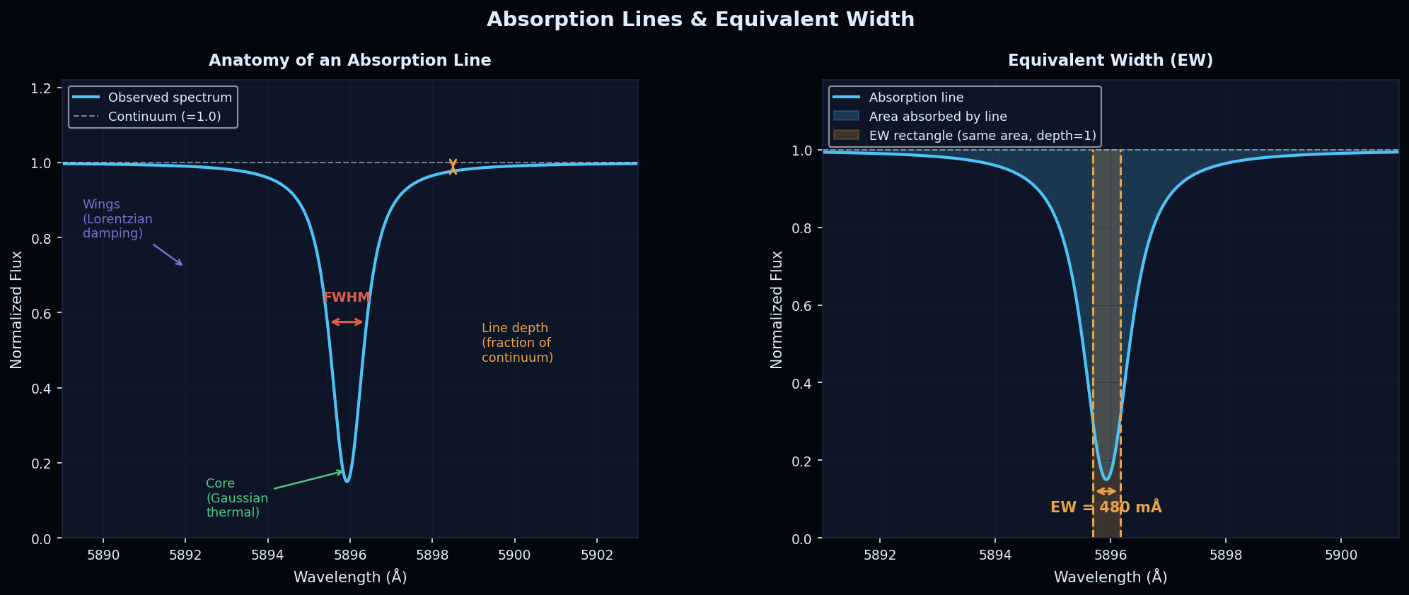
The distribution of electromagnetic radiation from an object, spread out by wavelength or frequency. A stellar spectrum shows how much light the star emits at each wavelength.
Think of it as a detailed "chemical fingerprint" of a star. Just as a supermarket barcode contains information encoded in bars of different widths, a stellar spectrum contains information about the star's composition encoded in the depths and positions of absorption lines.
Wavelength in Angstroms (Å) on x-axis; normalized flux (0 to 1) on y-axis
The HARPS spectrum of 55 Cancri A covers 3780–6910 Å at a resolution of R~115,000.
Absorption line, Continuum, Spectral resolution (R)
A dark feature in a stellar spectrum where atoms in the stellar photosphere have absorbed photons of a specific wavelength, removing that light from the outgoing beam.
Imagine a star's light as a full rainbow. Atoms in the outer layers of the star act like tiny "notch filters" — each element absorbs only its specific colours (wavelengths). The result is a rainbow with dark gaps at precise positions. Each gap is an absorption line, and each element has a unique set of gap positions — its spectral fingerprint.
Wavelength in Angstroms (Å)
The sodium D1 line at 5895.92 Å is one of the most prominent absorption features in the optical spectrum of a K-type star like 55 Cancri A.
Equivalent Width (EW), Continuum, FWHM
The smooth underlying flux level of a stellar spectrum, representing light from the photosphere unaffected by discrete atomic transitions. In a normalized spectrum, the continuum equals 1.0.
The "baseline" of the spectrum — the bright background against which dark absorption lines appear. Measuring a line's depth requires knowing the continuum level precisely. For metal-rich stars like 55 Cnc ([Fe/H]=+0.32), so many lines overlap that finding the true continuum is challenging.
Normalized flux (dimensionless, set to 1.0)
In the 5000–5400 Å region of 55 Cnc's spectrum, iron lines are so dense that the continuum must be estimated using model atmosphere predictions.
Normalization, Equivalent Width
A measure of the total absorption by a spectral line, defined as the width (in Angstroms) of a rectangular notch with depth equal to 1 (complete absorption) that has the same area as the actual line profile.
The EW is a single number that captures "how much light does this line remove?" regardless of the line's shape. A line that removes a lot of light has a large EW. A faint line has a small EW. The EW is what we measure from the spectrum to eventually calculate how much of each element is present.
Angstroms (Å) or milliAngstroms (mÅ). 1 Å = 1000 mÅ. Most lines: 5–300 mÅ.
The Na I D1 line in 55 Cnc has EW ≈ 480 mÅ (strong). A typical Fe I line has EW ≈ 50–80 mÅ (moderate). A P I line has EW ≈ 12 mÅ (weak — needs high S/N to detect).
Absorption line, Gaussian profile, Voigt profile, Curve of growth
The width of a spectral line measured at half the maximum line depth. A standard measure of line sharpness.
If a line's deepest point is 0.3 (flux = 0.3 below continuum = 1.0), the FWHM is the wavelength width measured where the line depth equals 0.3/2 = 0.15. Narrower lines (small FWHM) are easier to measure and less likely to blend with neighbouring lines. Used in the EW uncertainty formula: σEW ≈ 1.5 × FWHM / S/N.
Angstroms (Å)
A typical HARPS Fe I line has FWHM ≈ 0.08–0.12 Å. The Na D lines have FWHM ≈ 0.5–1.0 Å due to their strong pressure-broadened wings.
Broadening, Spectral resolution
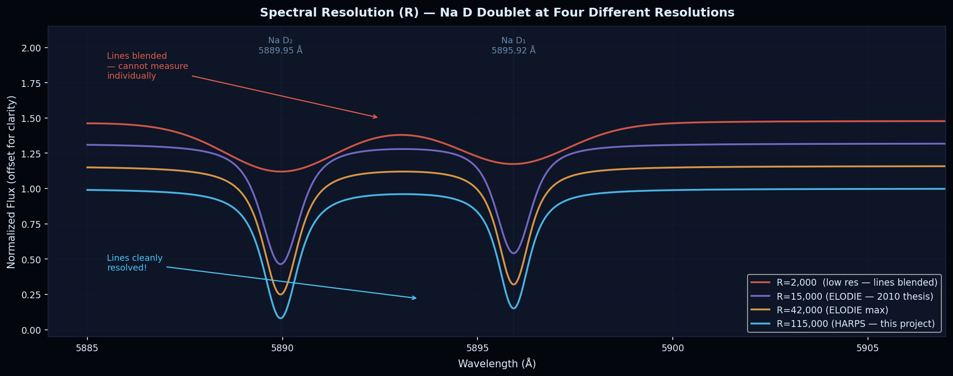
A dimensionless number defined as R = λ / Δλ, where λ is the wavelength and Δλ is the smallest wavelength difference the instrument can separate. Higher R = sharper, more detailed spectra.
Resolution tells you how close together two spectral features can be while still appearing as two separate lines. At R = 115,000 (HARPS), two lines just 0.05 Å apart can be distinguished. At R = 42,000 (ELODIE, used in 2010), lines must be 0.14 Å apart to be separated. This is why HARPS gives us 3× better detail.
Dimensionless ratio
HARPS: R~115,000. ELODIE (2010 thesis): R~42,000. The [O I] 6300.304 Å line and its Ni I 6300.336 Å blend are only 0.032 Å apart — only resolved at R > 100,000.
HARPS, ELODIE
Section 2
Codex Architecture
These terms describe how the Codex checks results, freezes references, and keeps the scientific record honest. Entries are alphabetical.
The distinction between abundances calculated with a one-dimensional atmosphere and non-local thermodynamic equilibrium corrections, and those calculated with a three-dimensional atmosphere and the same physics. The Codex applies a ratified 1D-to-3D correction to iron. Other metals remain on the 1D-NLTE scale until matching grids exist. Ratified by RYA-553; broader grid work is deferred to RYA-550.
A guard in pipeline/provenance_honesty.py that refuses to publish a “no independent-gf line survives” claim when a row has surviving lines or a measured value. The verdict emitter and gold-reference builder share the guard. It prevents a measured result from hiding behind a false blank cause. Ratified by RYA-596 and RYA-653.
The mutable state ledger. Every state-changing pull request updates it. A register-freshness guard blocks a pull request that changes a state surface without updating the register. Ratified by RYA-659.
An alternative acceptance gate for cases where ionization balance stops on precision rather than value. The rule has five bounded criteria and lives in docs/SCIENCE_STANDARDS.md. Titanium with the Mallinson 2024 atom was its first use. Ratified by RYA-545.
A loud-fail guard in pipeline/engine_selection.py. It raises when per-line winner selection produces a material disagreement between Engine A and Engine B at the element level. This prevents silent averaging.
A machine-generated, per-element report at data/audit/element_disposition_report.json. It reads the current phase_c verdict, gold reference, two-engine artifact, and tracker. It classifies each element as PASS held, PASS candidate, provisional flip, owed with cause, or data-gap. The report runs before every freeze and is not hand-editable. Ratified by RYA-663.
The analyst-facing state table at data/audit/element_status_tracker.csv. It is generated from the phase_c verdict, config/physics_regime_rya400.yaml, and an editorial sidecar. Hand-editing the CSV breaks the build. Ratified by RYA-654.
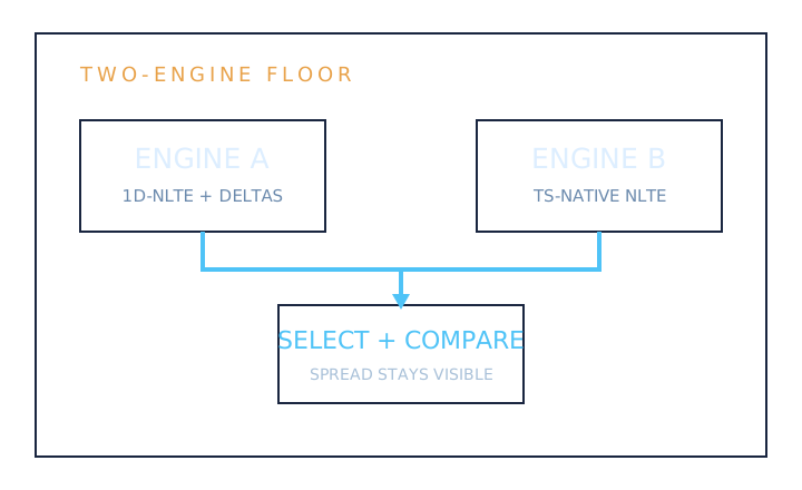
The 1D-NLTE production path. It measures an equivalent width or uses synthesis-v2, then applies a per-line NLTE correction from a one-dimensional correction table. The table may come from PySME-derived, MPIA, Korotin, INSPECT, or nlte_cno data. Engine A supplies the reported gold-reference value for most elements. Ratified by RYA-525.
The Turbospectrum-native NLTE synthesis path. It runs per line with the Gerber TS-native NLTE deck and uses native departure coefficients where a validated model atom exists. It runs beside Engine A for cross-engine verification. Ratified by RYA-533 and RYA-525.
The rule that state artifacts use one of four nouns: Catalog for a master enumeration, Register for mutable state facts, Tracker for work or progress, and Reference for frozen validated truth. “Gold” is reserved for a Reference modifier. Ratified by RYA-631.
A frozen, hashed, write-once solar abundance reference at data/reference/solar/solar_abundances_vN.csv. It is promoted from a phase_c verdict with scripts/promote_solar_reference.py --apply. A correction creates vN+1 rather than editing a frozen file. data/reference/solar/CURRENT names the active version.
Synthesis in which an atomic line is expanded into its hyperfine-structure components before fitting. The Codex uses it for Mn, Co, Cu, V, Sc, Ba II, Eu II, Na, and Al. Lithium at 6707 Å is not used as an HFS test in warm F stars because depletion can mimic a synthesis failure. Ratified by RYA-269.
A correction that is safe to request more than once because the pipeline recognizes an already-corrected state. The iron 1D-to-3D correction checks method_scale, so re-emitting cannot apply it twice. Ratified by RYA-553.
A continuous-integration guard that compares the element status tracker, phase_c verdict, and gold reference. It reports any disagreement that lacks a documented ratified divergence. Zero undocumented failures is the target. Ratified by RYA-632.
The repository-root startup index. It names the canonical register, tracker, catalogs, holdings manifest, and SEQUENCE.md read-set. Every session begins by reading that set. Every state-changing pull request updates at least one member. Ratified by RYA-659.
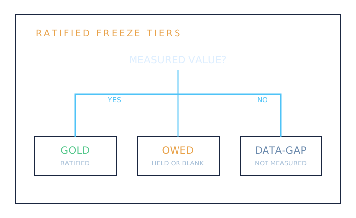
A ratified freeze tier that carries no frozen value even when the phase_c verdict contains a measurement. It is used when a value exists but has not been approved as gold-frozen. “Owed-HELD” and “owed-BLANK” are different states. Ratified by RYA-522.
The distinction between a measured value held from promotion and an element with no measurement. owed-HELD means the verdict contains a value that is not yet gold. owed-BLANK means no value has been measured. The blank-cause honesty tripwire keeps the states separate. Ratified by RYA-596.
The canonical per-element abundance verdict produced by scripts/phase_c_verdict_rya371.py. It combines equivalent-width measurements, NLTE corrections, dedicated synthesis channels, and ratified corrections. Each element has one row with its abundance, method, tier, and verdict status. Gold references are built from this channel.
A per-element classification in config/physics_regime_rya400.yaml. It distinguishes elements measured by equivalent width from elements sourced by synthesis. The tracker generator uses it to separate a verifier’s blind spot from a true measurement gap. Ratified by RYA-654.
A per-element assignment of gold, owed, or data-gap. It controls whether a phase_c verdict value is promoted into the frozen reference. Ryan ratifies each assignment; the computation does not. Ratified by RYA-522.
Elements that the phase_c verifier reports as having no measurement even though a synthesis or Kitt Peak atlas channel carries a real value. Co, N, K, and Cu are registered in data/audit/known_verdict_divergences.yaml and pinned by test. They are annotated divergences, not measurement gaps.
Two families of hydrogen-collision recipes in NLTE model atoms. Scaled-Drawin recipes are empirical and can overpredict corrections. Ab-initio recipes derive the collision physics directly and are often smaller. The model-atom vintage audit records which family each element uses and whether the difference is material. Ratified by RYA-546.
The per-star release deliverable. Each released star receives one PDF with twelve standard sections covering identity, provenance, parameters, abundances, science products, cross-region checks, anomalies, line diagnostics, uncertainty, caveats, data provenance, and method provenance. Each package is write-once, hashed, and versioned with its gold reference. Ratified by RYA-668.
The newest-first landing log at the repository root. Each merged ticket gets one line stating what landed and what it unblocks. It is a narrative overlay on the register, not a state machine. Ratified by RYA-666.
The HP ProBook 450 that serves as the authoritative production runner. Abundance computation and continuous-integration tests run there. The Mac is used for research, development, and pull-request review, not production computation. Ratified by RYA-517 and RYA-567.
A file listed in pipeline/state_surfaces.py. Changing one triggers the register-freshness guard. Examples include the verdict generator, gold builder, config/stars.yaml, and config/constants.py.
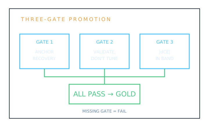
The strict test for promoting an element from owed to gold. Gate 1 requires Engine B to recover the external anchor within 0.05 dex. Gate 2 requires the model atom to pass the validate-don’t-tune firewall. Gate 3 requires the absolute dCE to remain within its band against the two-engine artifact. All three gates must pass. A missing gate fails. Ratified by RYA-561.
The architecture that runs Engine A and Engine B for every element with a validated model atom. Cross-engine spread is reported as a diagnostic and is never silently averaged into the result. CROSS_ENGINE_MIX_GATE flags a material conflict between per-line selection and element-level aggregation. Ratified by RYA-525.
The Codex firewall that forbids tuning an atom or grid to reproduce an anchor. The physics must produce the anchor. The anchor tests the model; it is not the model’s target.
Section 3
Line Profiles and Broadening
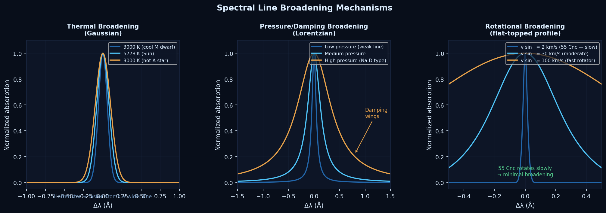
Real spectral lines are not infinitely sharp — they are broadened by several physical mechanisms. Understanding broadening is essential for choosing the right profile model (Gaussian vs Voigt) and for measuring accurate equivalent widths.
Broadening of a spectral line caused by the random thermal velocities of atoms in the stellar photosphere. Atoms moving toward/away from us Doppler-shift the absorbed wavelength, smearing the line into a Gaussian shape.
Imagine a thousand sodium atoms all absorbing light at 5895.92 Å. But they're not sitting still — they're moving randomly (thermal motion). Atoms moving toward us absorb slightly bluer wavelengths; atoms moving away absorb slightly redder ones. The result: absorption is spread over a small wavelength range, creating a bell-curve (Gaussian) shaped line.
Wavelength (Å); characterized by Gaussian σ or FWHM
For 55 Cnc (Teff = 5196 K), thermal broadening gives σthermal ≈ 0.07–0.10 Å for typical lines.
Gaussian profile, FWHM, Voigt profile
Broadening caused by collisions between the absorbing atom and surrounding gas particles, which perturb the atom's energy levels and allow absorption over a range of wavelengths. Creates Lorentzian-shaped wings extending far from the line centre.
When sodium atoms collide with neighbouring hydrogen and helium atoms thousands of times per second in the dense photosphere, the collisions momentarily shift the energy levels, allowing absorption at wavelengths slightly offset from 5895.92 Å. This creates broad "wings" on either side of the line core. The Na D lines are extreme examples — their wings extend ±3 Å from centre.
Wavelength (Å); characterised by damping constant γvdW (van der Waals)
Na D lines (EW ≈ 480 mÅ): heavily damped, broad wings. A weak Fe I line (EW ≈ 50 mÅ): negligible damping wings. Voigt profile required for lines with EW > 150 mÅ.
Voigt profile, Lorentzian, Damping constant
A bell-curve shaped line profile: F(λ) = 1 − A × exp(−½((λ−λ₀)/σ)²). Describes lines dominated by thermal and instrumental broadening.
The same bell curve as a normal distribution in statistics. For weak lines (EW < 80 mÅ), the Gaussian is an excellent approximation because thermal broadening dominates. For strong lines (Na D, Mg b), the Gaussian misses the pressure-broadened wings and underestimates the EW by up to 25%.
Depth A (dimensionless, 0 to 1), width σ (Å)
A Fe I line at 5328 Å with EW = 75 mÅ: well-fitted by Gaussian. Error vs Voigt < 2%.
Voigt profile, Lorentzian, Thermal broadening
A profile with broader, slower-decaying wings than a Gaussian: L(x) = 1/(1 + (x/γ)²). Describes lines dominated by pressure/damping broadening.
Named after physicist Hendrik Lorentz. Falls off as 1/x² instead of the Gaussian's exp(−x²) — much slower. This captures the damping wings of strong lines. However, a pure Lorentzian overestimates the core depth. The correct profile for stellar lines is the Voigt (convolution of Gaussian + Lorentzian).
Half-width γ (Å)
The damping wings of Na D extend several Angstroms — clearly Lorentzian in shape.
Gaussian profile, Voigt profile, Pressure broadening
The mathematically correct line profile for stellar absorption lines: the convolution of a Gaussian (thermal + instrumental broadening) and a Lorentzian (pressure/damping broadening). Implemented efficiently using the Faddeeva function.
For weak lines, the Voigt profile automatically reduces to a Gaussian (the Lorentzian component is negligible). For strong lines, the Voigt profile captures the broad wings that a pure Gaussian misses. This is why we use Voigt as our standard fit for all lines with EW > 80 mÅ.
Four parameters: amplitude, centre wavelength (Å), Gaussian FWHM (Å), Lorentzian FWHM (Å)
Na D1 at 5895.92 Å: Voigt fit with fwhmG ≈ 0.16 Å, fwhmL ≈ 0.40 Å. EW ≈ 480 mÅ. Using Gaussian instead would give EW ≈ 360 mÅ — 25% too small.
Gaussian profile, Lorentzian, EW, Damping
Broadening caused by stellar rotation. The near limb moves away from us; the far limb moves toward us. Both absorb at slightly different wavelengths, broadening lines and flattening their tops.
A spinning star has one edge moving toward you (blueshifted) and the other edge moving away (redshifted). Both edges have the same absorption lines, but shifted in opposite directions. The result is a line that appears wider and more flat-topped. v sin i is the rotation speed times the sine of the inclination angle (how tilted the rotation axis is relative to our line of sight).
km/s
55 Cancri A: v sin i = 2.3 km/s — very slow rotator. Rotational broadening is negligible. The Sun: v sin i ≈ 2 km/s. A hot A-type star like Vega: v sin i ≈ 20 km/s — significantly broadened.
FWHM, Spectral resolution
Section 4
Stellar Parameters
Four numbers completely describe the model atmosphere of a main-sequence FGK star. Getting these right is fundamental — errors in stellar parameters propagate into every elemental abundance we measure.
The temperature of a perfect blackbody that would emit the same total power as the star. In practice: the temperature of the outer photosphere where visible light escapes.
Teff is the single most important parameter for a star. It determines which atoms are ionized vs neutral, which controls which absorption lines appear. A star at 5196 K (55 Cnc) looks slightly more orange than the Sun (5778 K) because it emits relatively more red light. Hotter = bluer = more energetic photons.
Kelvin (K)
55 Cnc: Teff = 5196 ± 24 K (from CHARA interferometry). Sun: 5778 K. A-type star Vega: 9600 K.
Spectral type, log g, Model atmosphere
The base-10 logarithm of the gravitational acceleration at the stellar surface, in cgs units (cm/s²). Determines atmospheric pressure, which affects line widths and the balance between neutral and ionized atoms.
A higher log g means stronger gravity at the surface → denser, higher-pressure atmosphere → more collision broadening → stronger damping wings. For dwarfs (log g ≈ 4.4) vs giants (log g ≈ 2.0), the same spectral line can look completely different. We use Fe I vs Fe II balance to determine log g (see §4.2 of methodology).
log10(cm/s²) — "dex" (dimensionless logarithm)
55 Cnc: log g = 4.41. Sun: log g = 4.44. A red giant: log g ≈ 2.0 (much lower pressure).
Teff, Ionization equilibrium, Fe I, Fe II
A velocity parameter representing small-scale, non-thermal motions in the stellar photosphere (convective turbulence). Typically 0.8–1.5 km/s for FGK dwarfs. Suppresses saturation of strong lines.
Even after accounting for thermal and rotation broadening, strong lines still appear broader than a pure thermal model predicts. This excess broadening is modelled as microturbulence — tiny swirling motions in the photosphere smaller than a mean free path. If ξ is wrong, strong lines and weak lines give different abundances. We derive ξ by requiring all Fe I lines, regardless of strength, to give the same iron abundance.
km/s (velocity)
55 Cnc: ξ ≈ 0.9 km/s (typical for K dwarfs). Sun: ξ ≈ 1.0 km/s.
Microturbulence check (§4.2), Curve of growth, EW
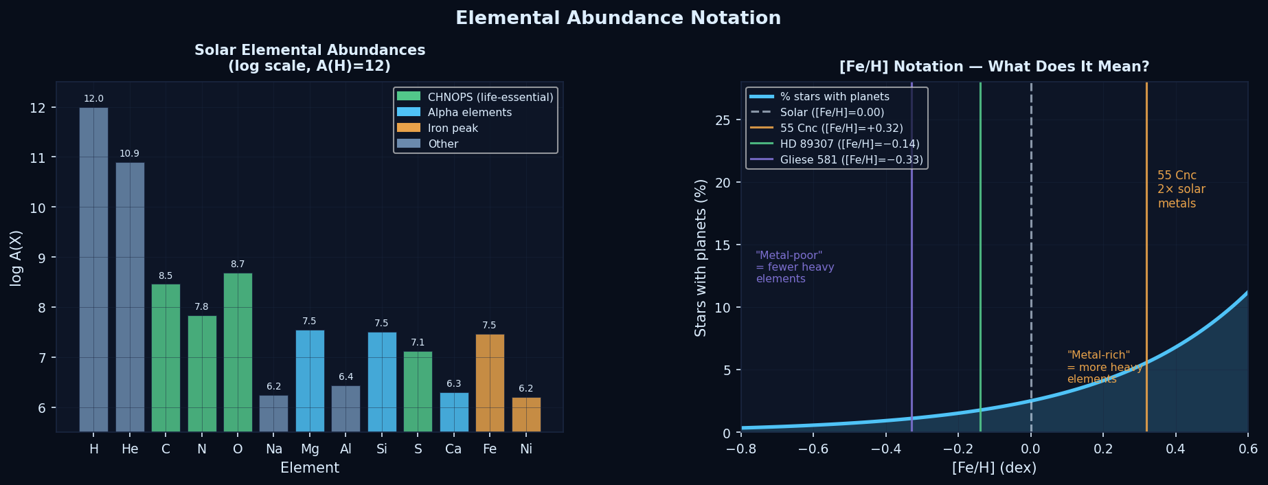
The logarithmic ratio of iron abundance in a star relative to the Sun. Used as a proxy for overall "metallicity" (abundance of all heavy elements). [Fe/H] = 0.00 by definition for the Sun.
[Fe/H] = log(NFe/NH)star − log(NFe/NH)Sun. Each +0.10 dex represents ~26% more iron than the previous level. +0.32 dex (55 Cnc) means roughly twice the solar iron abundance. Stars with more metals are more likely to host planets.
dex (dimensionless logarithmic ratio)
55 Cancri A: [Fe/H] = +0.32 (metal-rich — twice solar). Sun: [Fe/H] = 0.00. HD 89307: [Fe/H] = −0.14 (slightly metal-poor). Gliese 581: [Fe/H] = −0.33.
Metallicity, [X/H], [X/Fe], dex
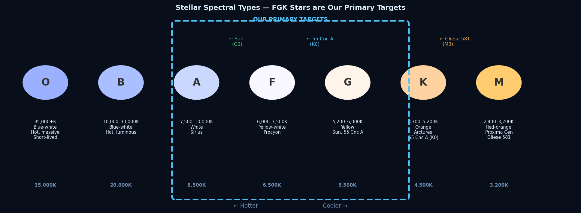
A classification system for stars based on their surface temperature and the pattern of absorption lines in their spectra. From hottest (O) to coolest (M).
The mnemonic "Oh Be A Fine Girl/Guy, Kiss Me" helps remember the sequence. Each type is subdivided 0–9 (e.g., G2 = slightly hotter than G5). The Sun is G2V — G-type, subtype 2, V = main sequence ("V" is Roman numeral 5, for luminosity class V).
Unitless classification
Sun: G2V. 55 Cancri A: K0IV-V. HD 89307: G0V. Gliese 581: M3V.
Teff, Main sequence
Section 5
Abundance Notation and Units
![Solar elemental abundances on the A(X) scale with CHNOPS, alpha, and iron-peak elements highlighted; and [Fe/H] metallicity-planet correlation](/assets/images/glossary/gloss_E.png)
Short for "decimal exponent." A logarithmic unit used throughout astronomy. A difference of 1.0 dex represents a factor of 10 in the actual quantity.
1.0 dex = factor of 10. 0.3 dex ≈ factor of 2. 0.1 dex ≈ factor of 1.26 (26% difference). So when we say [Fe/H] = +0.32, it means 55 Cnc has 100.32 ≈ 2.1 times more iron than the Sun.
Dimensionless (logarithmic)
[Fe/H] = +0.32 → factor of ~2.1 more iron than Sun. σ = 0.05 dex → ~12% uncertainty in actual abundance.
[Fe/H], [X/H], A(X)
The logarithmic abundance of element X on a scale where hydrogen = 12.00. Defined as A(X) = log(NX/NH) + 12, where NX and NH are the number of atoms per unit volume.
Why +12? Because hydrogen is the most abundant element in stars — about 1012 times more abundant than the least abundant elements. Adding 12 makes all abundances positive and manageable. A(H) = 12.00 always. A(Fe) = 7.46 for the Sun means roughly 1 iron atom per 35,000 hydrogens.
Dimensionless (logarithmic)
A(Fe)Sun = 7.46 (Asplund 2021). A(Na)Sun = 6.24. A(Fe)55Cnc ≈ 7.78 ([Fe/H] = +0.32 above solar).
[X/H], dex
The abundance of element X in a star relative to the Sun, on the logarithmic dex scale. [X/H] = A(X)star − A(X)Sun.
The brackets [ ] are standard notation for "abundance relative to the Sun." [Fe/H] = 0.00 means the same iron as the Sun. [C/H] = +0.20 means 60% more carbon than the Sun. This notation removes the very large A(X) numbers and focuses on differences from solar.
dex
[Fe/H] = +0.32 (55 Cnc iron). [Na/H] = +0.37 (estimated sodium). [O/H] = +0.12 (estimated oxygen — less enhanced than Fe).
[X/Fe], A(X), dex
The abundance of element X relative to iron (rather than hydrogen). [X/Fe] = [X/H] − [Fe/H]. Reveals nucleosynthetic patterns independent of overall metallicity.
If a star is metal-rich ([Fe/H] = +0.32), ALL elements tend to be more abundant — that's just what metal-rich means. [X/Fe] asks: "is element X enhanced or depleted RELATIVE to iron?" Alpha elements (Mg, Si, Ca) enhanced relative to iron ([α/Fe] > 0) means the star formed early in galactic history, before Type Ia supernovae had time to add iron.
dex
[Mg/Fe] = +0.05 for 55 Cnc: slightly enhanced Mg relative to Fe — typical for a mildly metal-rich K dwarf.
[X/H], Alpha-element enhancement, Galactic chemical evolution
The ratio of carbon to oxygen atoms in a stellar photosphere (or planetary composition). Solar C/O = 0.55. Below ~0.8: oxygen-rich chemistry (silicates). Above ~0.8: carbon-rich chemistry (SiC, graphite).
This is the most important single number for predicting rocky planet composition. On Earth, minerals like quartz (SiO2), olivine (Mg2SiO4), and feldspar dominate because oxygen is more abundant than carbon. If a star has C/O > 0.8, its planets might instead have silicon carbide (SiC) or graphite — possibly even diamond — instead of silicates. The contested C/O measurement for 55 Cancri (0.78 or >1?) is a primary science goal of this project.
Dimensionless ratio
Sun: C/O = 0.55. Earth crust: C/O ≪ 1 (oxygen dominant). Carbon planets (hypothetical): C/O > 0.8.
[C/H], [O/H], Planetary composition
Section 6
Model Atmospheres and LTE
A mathematical model of the physical conditions (temperature, pressure, density, opacity) in a stellar atmosphere as a function of depth, computed from equations of radiative transfer and hydrostatic equilibrium.
Without a model atmosphere, we can't convert an absorption line depth into an abundance — we wouldn't know the temperature and pressure conditions where the line was formed. ATLAS9 (Kurucz) provides pre-computed grids of model atmospheres parameterized by Teff, log g, [M/H], and ξ.
N/A — abstract mathematical model
ATLAS9 model for 55 Cnc: Teff=5196 K, log g=4.41, [M/H]=+0.32. Each model has 64 atmospheric layers with T, P, density at each depth.
ATLAS9, LTE, Teff, log g
The industry-standard grid of 1D, plane-parallel, LTE model atmospheres for FGK stars, developed by Dr. Robert Kurucz (Harvard) and updated by Castelli & Kurucz (2003). Used in the Exoplanet Codex pipeline.
ATLAS9 has been the backbone of stellar abundance analysis since the 1970s. The fact that it's still the standard in 2026 reflects how well the fundamental physics was captured. It's fast, well-tested, and matches observations of FGK dwarfs extremely well. MARCS (Sweden) is an alternative grid used for cross-validation.
N/A — software package and data grid
For 55 Cnc, we interpolate the ATLAS9 grid to exactly Teff=5196 K, log g=4.41. The model predicts how deep each absorption line should be for a given elemental abundance.
LTE, Model atmosphere, MARCS
The assumption that each small volume of the photosphere is in thermal equilibrium at the local temperature T, so that the Boltzmann and Saha equations correctly describe the distribution of atoms across energy levels and ionization states.
LTE is like assuming that every tiny parcel of stellar gas behaves as a perfect "black box" responding only to its local temperature — not to radiation from other layers or from outside the star. This is an excellent approximation in the dense photospheres of FGK dwarfs, where collisions are so frequent that local thermal equilibrium is maintained. It breaks down in low-density regions (chromosphere, corona).
N/A — physical approximation
LTE valid for: photosphere of FGK dwarfs, most absorption lines. LTE breaks down for: O I 7771–7775 Å triplet (requires NLTE correction of −0.20 to −0.40 dex); resonance lines of Na I, Li I.
NLTE, Model atmosphere, Saha equation
The condition where the radiation field or collisional rates are insufficient to maintain LTE, so the actual level populations differ from Boltzmann/Saha predictions. NLTE corrections are additive offsets applied to LTE abundances.
Some spectral lines form partly in the low-density outer photosphere where the radiation field (photons from deep inside the star) "pumps" atoms into higher energy states than thermal collisions alone would produce. This changes the line depth in ways the LTE model can't capture. We apply published NLTE correction grids (Amarsi et al. 2021) to fix this.
Correction in dex, typically −0.03 to −0.40 dex
O I 7773 Å: NLTE correction ≈ −0.30 dex. Na I D: −0.07 dex. [O I] 6300 Å: 0.00 dex (no correction needed — forbidden lines form under LTE).
LTE, Forbidden line, Amarsi et al.
A spectral transition prohibited under electric-dipole selection rules but occurring via magnetic-dipole or electric-quadrupole transitions. Denoted with brackets: [O I] for the forbidden oxygen line.
In high-density environments, atoms are constantly colliding and de-exciting before they can absorb via forbidden transitions. But the forbidden [O I] 6300.304 Å line can still form as an absorption line against the bright continuum. The key advantage: forbidden lines form strictly under LTE — no NLTE correction needed, making them cleaner oxygen abundance indicators.
N/A — type of atomic transition
[O I] 6300.304 Å: the most important forbidden line for stellar oxygen abundance work. Note: the Ni I blend at 6300.336 Å is only 0.032 Å away — a key systematic for C/O measurements.
LTE, NLTE, [O I], Ni I blend
Section 7
Nucleosynthesis and Element Groups
The elements in a star did not form in that star — they were forged in supernovae and other stars over billions of years of galactic chemical evolution. Understanding which process made each element explains the patterns we see in stellar abundances.
Elements with atomic masses that are integer multiples of the helium nucleus (alpha particle, mass 4): O, Ne, Mg, Si, S, Ar, Ca, Ti. Produced primarily by massive stars and Type II supernovae.
These elements are produced by alpha capture — successive fusion of helium nuclei onto heavier elements. They're called "alpha elements" because each step adds one alpha particle (helium nucleus). Since they come from short-lived massive stars, they were abundant early in galactic history. The ratio [α/Fe] tells us WHEN a star's birth cloud was enriched.
N/A — element classification
High [α/Fe] (e.g., +0.3) = old star formed before Type Ia SNe contributed iron. Low [α/Fe] (~0) = star formed after the galaxy was enriched with iron from Type Ia SNe. 55 Cnc has solar [α/Fe] — consistent with its ~10 Gyr age.
Iron-peak elements, Type II supernova, [α/Fe], Galactic chemical evolution
Elements near iron in the periodic table (V, Cr, Mn, Fe, Co, Ni, Cu) that have the highest nuclear binding energy per nucleon. Produced primarily by Type Ia supernovae. Also includes Al as a refractory rocky-planet tracer.
Iron is the "most stable" nucleus — you can't release energy by fusing iron into heavier elements or splitting it into lighter ones. Elements near iron share this high stability. Type Ia supernovae (white dwarf explosions in binary systems) are the primary source, enriching the galaxy with iron-peak elements over billion-year timescales.
N/A — element classification
Ni/Fe ratio in rocky planets predicts core composition. Co and Cr trace the relative contributions of Type Ia vs Type II supernovae. Cu (odd-Z, bio-essential trace metal) is measured from Cu I 5105/5218 Å. Al (refractory, crustal composition) uses two weak lines at 6696/6698 Å — best-effort measurement.
Alpha elements, Type Ia supernova, [Fe/H]
The six elements essential for all known life: Carbon (C), Hydrogen (H), Nitrogen (N), Oxygen (O), Phosphorus (P), Sulfur (S). Their relative abundances in a star predict whether its planets could host life.
These six elements make up ~98% of all living matter on Earth. Carbon forms the backbone of organic molecules. Hydrogen and oxygen combine to make water. Nitrogen is in DNA and proteins. Phosphorus is in ATP (the cell's energy currency) and DNA. Sulfur is in amino acids. Phosphorus is now recognised as the LIMITING nutrient — it's the scarcest of the six in most stellar environments and varies by 10× across FGK stars.
N/A — element group acronym
The CHNOPS habitability index compares a star's C:N:O:P:S ratios to the "Redfield ratio" — the composition of marine organisms on Earth.
Habitability, Redfield ratio, P I lines
Elements heavier than iron formed by the slow neutron capture process (s-process) in AGB (Asymptotic Giant Branch) stars. Include Ba, Y, Zr, La, Ce, Nd.
When iron nuclei slowly capture neutrons (one at a time), with time between each capture for the nucleus to beta-decay, you build up s-process elements. This happens inside evolved giant stars. The ratio Y/Mg is a stellar "chemical clock" — young stars have more Y relative to Mg because more AGB stars have had time to enrich the galaxy.
N/A — nucleosynthesis process
Ba II 5853.67 Å is a strong, easily measurable s-process line. Y II 4883 Å traces galactic age.
r-process, Alpha elements, Galactic chemical evolution
Section 8
Pipeline and Analysis Terms
High Accuracy Radial velocity Planet Searcher. A spectrograph at the ESO 3.6m telescope, La Silla, Chile. Spectral resolution R~115,000, wavelength coverage 3780–6910 Å. The primary instrument for Exoplanet Codex spectroscopy.
HARPS was built to measure stellar radial velocities to 1 m/s precision — accurate enough to detect the wobble caused by an Earth-sized planet. This extreme precision requires high spectral resolution, which is exactly what we need for abundance work. It is also why we have 88 archival HARPS spectra of 55 Cancri — it was a prime target for planet searches.
R = λ/Δλ = 115,000 (dimensionless)
HARPS can resolve features separated by 0.05 Å at 5800 Å. ELODIE (used in 2010 thesis): R~42,000.
ELODIE, Spectral resolution, ESO archive
Space Telescope Imaging Spectrograph — a UV and optical spectrograph aboard the Hubble Space Telescope. Wavelength coverage ~1150–10,000 Å. Used in the Codex for UV spectral lines inaccessible from Earth's surface.
Earth's atmosphere absorbs ultraviolet light below ~3000 Å, blocking access to many important spectral lines of carbon, nitrogen, oxygen, and other elements. STIS on HST orbits above the atmosphere, providing access to these UV features. For 55 Cnc A, gratings G140M, G750L, G430L were used; for Alpha Cen A, the high-resolution echelle gratings E140H, E140M, E230H, E230M were used.
N/A — instrument
O I UV lines at ~1302 Å and C II at ~1335 Å are only accessible via HST/STIS — both blocked by the atmosphere at ground-based observatories.
HST/COS, MAST, Multi-wavelength analysis, HARPS
Cosmic Origins Spectrograph — a far-ultraviolet spectrograph aboard the Hubble Space Telescope. Wavelength coverage ~1150–3200 Å. Optimized for high sensitivity in the far-UV where STIS has lower throughput.
COS was installed on HST during Servicing Mission 4 (2009) specifically to boost sensitivity in the far-UV. It detects extremely faint UV features that would otherwise require impractically long exposure times. Used in the Codex where far-UV spectra are available and needed for element coverage.
N/A — instrument
Far-UV coverage ~1150–3200 Å includes Ly-α at 1216 Å and UV transitions of N, C, Si, and O not accessible from the ground.
HST/STIS, MAST, Multi-wavelength analysis
Mikulski Archive for Space Telescopes — NASA's archive for data from the Hubble Space Telescope and other space observatories. All HST spectra used in the Codex are retrieved from MAST.
MAST is to space telescope data what the ESO Science Archive is to ground-based data. It hosts the full HST archive — including all STIS and COS spectra — and provides free public access after a 12-month proprietary period. The Codex retrieves all HST data from mast.stsci.edu.
N/A — data archive
Alpha Cen A: ~111 HST observations retrieved from MAST spanning multiple programs and gratings (downloading as of May 2026).
HST/STIS, HST/COS, ESO archive
Combining spectra from multiple wavelength regimes — typically optical (HARPS, 3780–6910 Å) and ultraviolet (HST, ~1150–3200 Å) — to access elemental spectral lines unavailable in any single wavelength window.
No single spectrograph covers everything. HARPS gives excellent optical coverage but cannot see UV lines. HST/STIS and COS cover the UV but don't observe from the ground. By combining both data sets, we access a much wider set of element lines — including UV transitions of N, O, C, and S that are essential for the CHNOPS habitability assessment.
N/A — analysis strategy
For Alpha Cen A: HARPS provides 75 high-SNR optical spectra; HST STIS/COS provides UV coverage down to 1150 Å. Together they enable measurement of all 27 target elements including those with only UV spectral lines.
HST/STIS, HST/COS, HARPS, MAST, CHNOPS
The ratio of the signal (flux) to the noise (random fluctuations) in a spectrum. Higher S/N = cleaner, more precise measurements.
Every spectrum has noise — random fluctuations from photon counting statistics. S/N = 200 means the signal is 200 times the noise. For abundance work, S/N > 200 is the minimum; S/N > 400 is preferred. Weak lines like P I (EW ≈ 12 mÅ) require S/N > 300 for a reliable measurement.
Dimensionless ratio
55 Cnc single HARPS exposure: S/N ≈ 100. Co-added 88 spectra: S/N ≈ √88 × 100 ≈ 940.
Co-adding, Photon noise, EW uncertainty
The component of a star's velocity along our line of sight (toward or away from us). Measured from the Doppler shift of spectral lines. Must be corrected before co-adding spectra.
If a star moves toward us, all its spectral lines shift to shorter (bluer) wavelengths. If it moves away, they shift to longer (redder) wavelengths. The formula: Δλ/λ = v/c. 55 Cnc has a systemic RV of +27.58 km/s (receding at 27.58 km/s). Its 5-planet system causes additional RV variation of ±100 m/s — small but significant when co-adding spectra.
km/s
55 Cnc systemic RV = +27.58 km/s. At 5895 Å, this shifts all lines by: 5895 × 27.58/299792 ≈ 0.54 Å.
Doppler shift, Barycentric correction, Co-adding
A correction applied to observed wavelengths to remove the component of Earth's orbital motion along the line of sight to the star. Applied automatically by the ESO HARPS pipeline.
Earth orbits the Sun at ~30 km/s. Depending on the time of year and direction of observation, Earth is moving toward or away from the target star at up to ±30 km/s. This shifts all spectral lines by up to ±0.6 Å at 5800 Å. The barycentric correction transforms wavelengths to what would be measured from the solar system barycentre (centre of mass).
km/s velocity correction; Angstroms wavelength shift
The ESO HARPS pipeline applies the barycentric correction to all S1D spectra automatically — we only need to apply the stellar systemic RV correction separately.
Radial velocity, Doppler shift
The relationship between the equivalent width of a spectral line and the abundance of the absorbing element. Has three regimes: linear, flat (saturated), and damping.
If you add more iron atoms to a stellar atmosphere, iron lines get deeper. But the relationship is not simple. Weak lines grow linearly with abundance (more atoms = proportionally deeper). Strong lines saturate (the core is already black — adding more atoms doesn't help). Very strong lines eventually grow again via pressure-broadened wings. The curve of growth tells us which regime each line is in.
Axes: log(abundance) vs log(EW/λ) (both dimensionless)
Fe I at 5328 Å (EW=75 mÅ): linear regime. Na D (EW=480 mÅ): damping regime. A flat-part line: sensitive to microturbulence ξ.
Equivalent width, Microturbulence, Voigt profile
The primary online database for atomic and molecular spectral line data, providing wavelengths, excitation potentials, oscillator strengths (log gf), and damping constants for hundreds of millions of spectral transitions.
VALD3 is to stellar spectroscopists what NIST Standard Reference Materials are to chemists — the authoritative source for atomic data. Before we can calculate abundances from an EW measurement, we need to know the transition probability (log gf) of that line. VALD3 provides this for every line we use.
N/A — online database
For 55 Cnc, we submitted an "Extract Stellar" request to VALD3 with Teff=5196 K, log g=4.41, threshold 0.001, HFS enabled, returning ~125,000 transitions across 3780–6910 Å for 27 target elements (includes hyperfine structure components for Ba, Eu, Li, Mn).
log gf, NIST, Excitation potential
The logarithm of the product of the statistical weight (g) and the oscillator strength (f) for an atomic transition. Determines the transition probability — how likely an atom is to absorb a photon of that wavelength.
log gf is the "volume knob" for how strong a spectral line is. A high log gf (e.g., 0.0) means a highly probable transition — a strong line. A low log gf (e.g., −5.0) means a very improbable transition — a weak line. Poorly known log gf values are a major source of systematic uncertainty in abundance work — we only use NIST grades A and B.
Dimensionless (logarithmic)
Na I D1: log gf = −0.184 (NIST grade A+). Fe I at 5328 Å: log gf = −1.466 (NIST grade A). [O I] 6300 Å: log gf = −9.717 (forbidden line — very weak transition probability).
NIST quality grades, Oscillator strength, EW
Quality grades assigned by the National Institute of Standards and Technology to oscillator strength (log gf) measurements, based on their estimated uncertainty.
Not all log gf values are equally reliable. NIST grades each value: A+ (<1% uncertainty), A (<3%), B (<10%), C (<25%), D (>25%). We only use grades A+, A, and B in the Codex pipeline. Using a grade C or D log gf value could introduce a 0.1–0.3 dex systematic error — swamping our actual measurement precision.
Letter grade (A+, A, B, C, D)
We measure ~200 lines total but include only ~140 in our primary analysis after filtering for NIST grade ≥ B.
log gf, Systematic uncertainty, NIST
Section 9
Key Science Outputs
The ratio of magnesium to silicon abundance in a stellar photosphere, used to predict the dominant silicate minerals in rocky planets.
Magnesium and silicon are the two main ingredients of rock-forming silicates. Their ratio determines the mineral balance: Mg/Si > 1 → olivine-dominated mantle (Mg2SiO4, like Earth's upper mantle). Mg/Si < 1 → pyroxene-dominated (MgSiO3). This directly predicts whether an exoplanet would have an olivine or pyroxene-rich interior — which affects volcanism, plate tectonics, and habitability.
Dimensionless atomic ratio
Sun: Mg/Si = 1.05. Earth: Mg/Si ≈ 1.02. Mars: Mg/Si ≈ 0.95. 55 Cnc A: Mg/Si ≈ 0.93 (literature) — slight pyroxene tendency.
C/O ratio, Fe/Si, Rocky planet composition
The ratio of iron to silicon abundance, used to predict the core mass fraction of rocky planets.
Iron sinks to the core during planetary formation (iron is denser than silicates). Higher Fe/Si in the host star means more iron in the planet, and therefore a larger iron core relative to the mantle. Earth's Fe/Si is higher than solar because of core formation — a large iron core (32% of Earth's mass) concentrated the iron.
Dimensionless atomic ratio
Sun: Fe/Si = 0.86 (by mass). Earth: Fe/Si = 1.69 (enriched due to large core).
Mg/Si, C/O ratio, Core mass fraction
The mean enhancement of alpha elements relative to iron: [α/Fe] = mean([Mg/Fe], [Si/Fe], [Ca/Fe], [Ti/Fe]). A tracer of galactic chemical evolution and stellar age.
Early in the Milky Way's history, only massive short-lived stars had died, producing alpha elements but little iron. Over time, Type Ia supernovae (which take ~1 billion years to explode) added large amounts of iron, gradually lowering [α/Fe]. Old stars (formed early) have high [α/Fe]; young stars (like the Sun) have near-solar [α/Fe].
dex
55 Cnc ([α/Fe] ≈ 0): solar-ratio alpha elements — typical for a 10 Gyr old thin-disk star. Metal-poor halo stars ([α/Fe] ≈ +0.4): very old, formed before Type Ia SNe.
Alpha elements, Type Ia supernova, Galactic chemical evolution
A quantitative score comparing a star's measured C:N:O:P:S abundance ratios to the "Redfield ratio" — the elemental composition of marine organisms on Earth. Provides a normalised measure of bio-essential element availability.
Life on Earth needs certain elements in approximately certain ratios. The Redfield ratio (C:N:P = 106:16:1 in marine organisms) is the starting point. By comparing a star's CHNOPS ratios to this biological benchmark, we get a number that captures "how well does this system's chemistry match the chemistry of life?" A score of 1.0 = identical to Redfield. Scores < 1.0 indicate depletion in one or more bio-essential elements.
Dimensionless index (Redfield-normalised)
A star depleted in phosphorus by 10× relative to carbon would score poorly on the CHNOPS index even if C, N, O, and S look fine — because P is the limiting nutrient.
CHNOPS, Redfield ratio, P I lines, Astrobiology